How does proportional CPU allocation work with AWS Lambda?
Originally appeared on Opsgenie Engineering Blog
We have been using AWS Lambda for over two years at OpsGenie. Our primary programming language for our Lambda functions is Java. Although Java tends to use more memory compared to other languages such as Node.js and Python, we still allocate more memory than we need for our functions. There are two primary reasons. Sometimes depending on the traffic, there can be unexpected spikes in usage. These spikes can cause out of memory exceptions. We prefer to allocate more memory instead of experiencing these errors in production. Second reason is, although you only specify the RAM, AWS allocates proportional CPU to your functions. For instance, AWS allocates twice much CPU power for your function while going from 128MB to 256MB of RAM. However, AWS Lambda supports 3GB of memory. Since the CPU power is proportional to RAM, you may think that 3GB function is 24 times faster than the 128MB function. But, the 3GB Lambda does not have 24 CPUs. Even if it did, it would be expensive as hell and wouldn’t be beneficial for many people since most of the code can’t make use of parallelism in an effective manner.
How does AWS allocate proportional CPU for your function?
There is no such thing as 1⁄10 CPU, you can not physically divide 1⁄10 of the CPU. But, you can allocate 1⁄10 of the time of the CPU to a single function, and you can have 10 of them working at the same time to share the same CPU core.
This concept is nothing new, it is called “time-sharing”. During 1960s, when people were using mainframes and the CPU power was expensive, each user was allocated fixed times so that the large mainframe could be shared among many people. The concept evolved over the years and operating systems now have schedulers that are responsible for scheduling many processes. One of the popular ones is Completely Fair Scheduler (CFS) which was merged in 2007 into the Linux Kernel. Basically it accounts the CPU usage of processes and tries to be fair among many processes. Therefore, in your computer, even if you have a single-core CPU, while you can zap on the web browser for cute cat pictures, Spotify can play its music at the background. Applications share the system’s CPU power in microsecond intervals.You don’t notice the switches since you are a nice human that has response time in the millisecond range. If you were to type “_ps aux_” in terminal or open Task Manager / Activity Monitor, you would see hundreds of processes working together and you don’t even notice lags unless the system is highly loaded.
Since it is possible to schedule many processes in a single system, it is also possible to set constraints on the scheduling algorithms. Although operating system tries to be fair as much as possible, it does not limit the total usage. So, if there is no one requesting CPU, the greedy one would get it as much as it likes. If you are paying for these resources, or you are renting it to customers like service providers such as Amazon, you would not like rogue processes that try to consume all the power. Even though the schedulers try to be fair, there is no guarantee that they can remain fair all the time, due to many reasons such as high load, or unpredictable behavior such as IO. Therefore, putting constraints on how much the CPU can be used is a good idea.
To better understand how it works, we will use a Docker image with a single task doing some useless encryption that takes significant amount of time. At the end, you will be able to see how the runtime performance is affected by the throttling constraints.
In detail, the example code is running bcrypt algorithm on a random set of bytes for a defined number of iterations in each batch. Since each invocation takes microseconds of time, we will run the algorithm for a number of iterations to get a less noisy result. We will use a c5.xlarge EC2 instance, which has 2 CPUs and install Docker with the test image we created. To improve the results and reduce the errors, we will run the code for many iterations. Thanks to Golang, Docker image is just 2.5MB, meaning you can easily play with it in your own environments.
Running it without any restriction, it gives the following output for batch size of 50 and 5 iterations:
$ docker run -ti mustafaakin/bench -batch 50 -iterations 5

{
 "Durations": [
  52,
  52,
  52,
  52,
  52
 ],
 "Mean": 52,
 "Variance": 0,
 "StdDev": 0,
 "CoefficientOfVariation": 0,
 "Max": 52,
 "Min": 52,
 "NoOfCores": 2
}
Each iteration elapsed 52 milliseconds, and there is no variance in the execution. Docker has two flags, which sets the scheduler period and the allowed quota for a given function by assigning the limits to the Cgroup of the running container:
$ docker run --help

 — cpu-period int Limit CPU CFS (Completely Fair Scheduler) period
 — cpu-quota  int Limit CPU CFS (Completely Fair Scheduler) quota
If the values are set, a running container is only allowed for running for quota microseconds in the given period. So, if you want 10% utilization, you can say your function has a quota of 1 millisecond for each 10 milliseconds. Therefore, if it consumes 1 millisecond of CPU, it has to wait for another 9 milliseconds to be able to execute again. The periods are in microseconds and an example invocation can be seen as follows:
$ docker run — cpu-period=10000 — cpu-quota=1000 -ti mustafaakin/bench -batch 50 -iterations 5

{
 "Durations": [
  520,
  556,
  529,
  520,
  520
 ],
 "Mean": 529,
 "Variance": 194.4,
 "StdDev": 13.94,
 "CoefficientOfVariation": 0.026,
 "Max": 556,
 "Min": 520,
 "NoOfCores": 2
}
What happens in multi-core case? Even if you have 2 CPUs and some code that can work in parallel, when you set the same period and quota as above, you will still get the same performance. Because, if your process runs for 10 seconds and utilizes all of the 2 CPUs, your process consumes 20 seconds of CPU time.
As you see, the mean of each batch performance is reduced by 9.8% of the unconstrained version. However, the variance in mean duration increases. CoefficientOfVariation variable is the standard deviation divided by mean, which normalizes the standard deviation and gives a rough idea of the severity of the variation compared to the mean. This metric is important, since if you allow your function to work for a limited amount of time, it will get continuously throttled, and swapped with other processes. This constant context-switching introduces an overhead since the proper kernel structures must be created and the process state must be preserved. On the other hand, if your period is very large, your function might not even be active for the whole period. For instance, a realistic Lambda function will probably wait for an I/O on an external system, hence your function will end early, and it will not be throttled. In short, for proper throttling, your period and quota should be set on a sweet spot where you do not have an overhead and also guarantee the Quality of Service (QoS).
How does this all fit in AWS Lambda?
AWS Lambda just started supporting Golang. As you can run native binaries in Golang, you can have uniform and more predictable executions compared to other languages. This is one of the reasons why this experiment is conducted now. We will use the exact same code and run it in AWS Lambda starting from 128MB, with 64MB increments. The batch value will be 100 so that we don’t have significant variations. We will also try 1, 2, 3 and 4 threads which are simultaneously trying the same thing. In other words, threads are not to decrease the time, but to increase the work.
You can verify that AWS Lambda uses Cgroups for CPU throttling by reading the contents of the special file /proc/self/cgroup and see your function is assigned to specific control groups such as “2:cpu:/sandbox-root-UXXIp3/sandbox-023d01”, but you cannot directly see the imposed limits. There are other resource types which can be throttled, if you are interested Linux kernel has an extensive documentation on them.
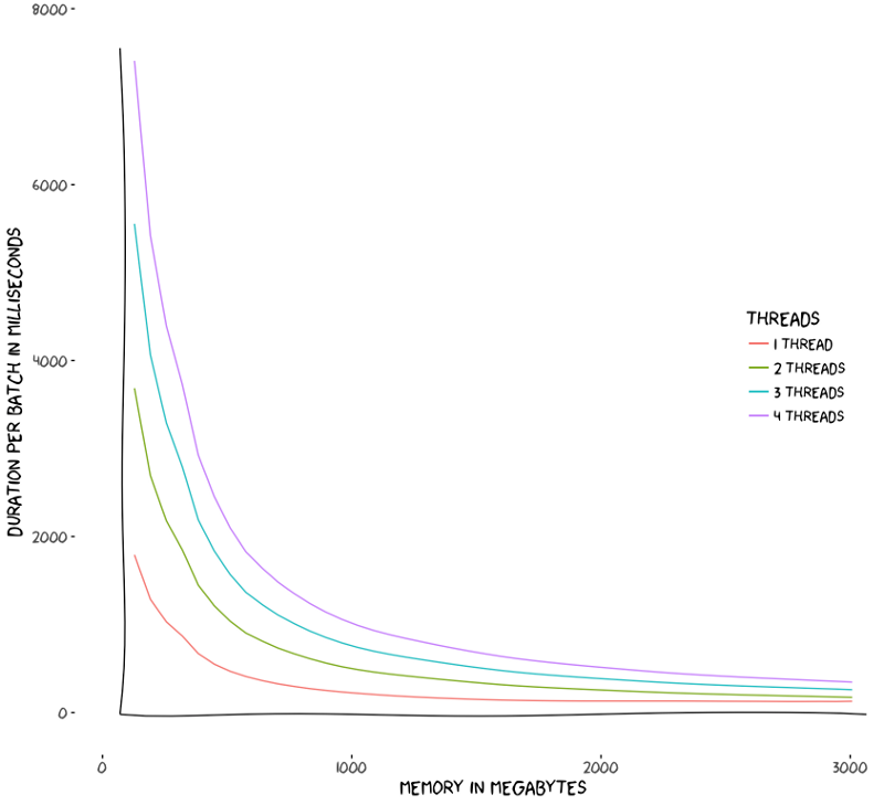
As expected, when memory size increases, the total time decreases. It means AWS keeps its promise and gives proportional CPU to your function. However, the above chart does not explain it in detail. It would be better if we drew it in in logarithmic scale, since the resulting time reduces exponentially as the memory is incremented with 64MB intervals. But, to better put things into perspective, we created another plot. Since AWS charges you by the total time multiplied by memory of your function, it is natural to want to see how much you pay for your function for various memory configurations.
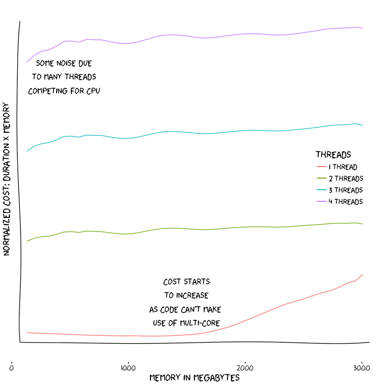
As it can be seen from the above figure which plots memory vs normalized cost, since our task is CPU-bound, we see that as the memory increases, we don’t have significantly increasing cost, since CPU power also increases proportionally. In other words, if your function completes in 30 seconds with 512MB RAM, it should complete around 15 seconds with 1GB of RAM. However, there is an exception for one thread case where the cost starts to increase around 1.5GB RAM. This is due to AWS starting to allocate more than 1 CPU and our code not being able to make use of that since it is a single-threaded CPU task.
The function we used in this example run is heavily CPU-bound. In reality, you would have tasks that probably connect to other services. This introduces uncertainties on how the CPU is utilized over time due to waiting for bytes from a network connection. Therefore, the throttling of your functions will likely change over time. However, when you are doing extensive input processing, i.e. parsing the data received from a Kinesis stream, resizing an image submitted to S3, your function will be using CPU heavily and will be subject to throttling. Even if you are not doing major processing, establishing an HTTPs connection will consume some CPU due to encryption.
As a best practice, we recommend you to profile your application. This way, you can see where the bottlenecks are, whether you are IO-bound or CPU-bound, and then you can adjust your function configuration for ideal memory settings to achieve balanced response time and cost.